Basic Graphing Review

| Multimedia | Practice Homework | Homework |

Context

As we have discussed it is important to have basic graphing skills. This includes being able to:

1. create graphs from mathematical relationships and from experimental data,
2. read and interpret graphs,
3. predict the shapes of graphs given the mathematical relationship, and
4. identify basic mathematical relationships from graphs.

What is basic graphing?

Basic graphing is how to draw a graph from a data table and recognizing some characteristic shapes that graphs have in the physical sciences.

Explanation

As we have seen, graphs are separated into an x-axis, which is usually horizontal, and a y-axis, which is usually vertical. These axes are perpendicular, or at 90 degrees, with respect to each other. The range of values appropriate for the variable that is placed along the x-axis is evenly distributed along that axis. The same is done for the variable that is along the y-axis.

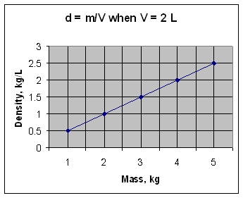
For a given value of the variable along x, the value of the variable along y can be calculated from a mathematical relationship. Consider the density relationship, d = m/V, when V = 2 L. If the mass is 1 kg, the density will be 0.5 kg/L. If the mass is 2 kg, the density will be 1.0 kg/L. And so on. The following table shows the calculated values of density (when V = 2 L) for a few different masses.

Mass in kg	Density in kg/L
1	0.5
2	1.0
3	1.5
4	2.0
5	2.5

If mass is placed along the x-axis and density is placed along the y-axis, then a graph like the one shown below can be generated by going along x to the value of one of the mass readings, and then going up along the y-axis to the corresponding y-value and putting an asterisk (*). This same process is repeated for each value of the mass. The corresponding density when mass is two is shown by a dashed line in the graph below. Similar lines could be drawn for each value of the mass. Reading a graph uses the same process in reverse. For a density of two, a horizontal line going through the value of two should be drawn across until it crosses the curve. A vertical line is then drawn downward through that intersection point until it crosses the x-axis. The value at that crossing point on the x-axis (4 kg) is the value of the mass corresponding to a density of two and a volume of 2 L.

This section will help you:

• Predict the shape of graphs given some fundamental mathematical expressions.
• Predict mathematical expressions from the shape of a graph.

Model

For our investigation of basic math we will only consider four common mathematical expressions (the examples are sample equations that have the corresponding proportionality):

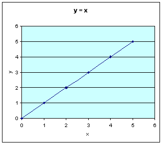
1. y Directly Proportional to x (e.g. y = x)

2. y Inversely Proportional to x (e.g. y = 1/x)

3. y Proportional to x-Squared (e.g. y = x²)

4. y Proportional to the Square-Root of x [e.g. y = √x also written as y = sqrt(x)]

Tables and their corresponding graphs are shown below for the first quadrant only (that is when both x and y are positive numbers). In this class we will only consider the first quadrant, but the reasoning will apply to other quadrants as well.

For y = x:

x y 1 1 2 2 3 3 4 4 5 5

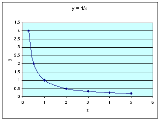
For y = 1/x:

x y 0.25 4 0.5 2 1 1 2 0.5 3 0.33 4 0.25

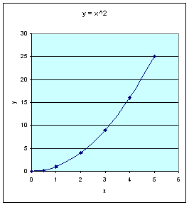
For y = x²:

x y 1 1 2 4 3 9 4 16 5 25

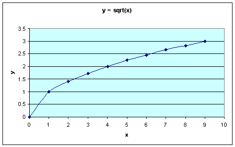
For y = √x:

x y 1 1 2 1.41 3 1.73 4 2 5 2.24 6 2.45 7 2.65 8 2.83 9 3

It is often the case that graphs are generated from experiment. It is important to be able to predict the shape of a graph and then be able to test the prediction experimentally. Consider an experiment to determine the distance traveled by an object moving at constant speed as the amount of time varies. What would be the shape of this curve? The word curve is often used loosely to include straight lines. From our experience it seems likely that the longer the object travels at a constant speed the farther the distance will be from the starting point. The graph would be predicted to look something like the one shown below. Notice that there are no numbers on the graph. It is the shape of the curve that is important at this point. As graphs are predicted, it is often advantageous to think about which of the four functions discussed above could produce the predicted graph. Which of the four functions discussed above could produce the predicted graph shown below?

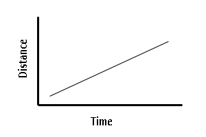
This is a straight line and so the example y = x, could result in this graph. A straight line can be expressed as y = mx + b. This is a general expression for any straight line. In this equation m and b are constants. For the example y = x; m = 1 and b = 0.

After predicting the shape of the experimental graph it is time to collect data and graph that data as outlined above. To graph distance versus time it is necessary to determine the distance at specified times. This could be done using devices to measure length (metersticks, etc.) and timers. Assume the data points on the graph shown below are from an experiment with a constant velocity of 0.4 m/s (meters per second). How close are the prediction graph and the experimental graph? Both graphs are basically the same, showing a Y directly proportional to X curve. The experimental graph allows a slope to be calculated, the prediction graph can be thought of as having different axis scales (which would change the apparent slope).

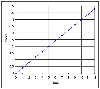
It is also important to be able to predict the mathematical relationship from graphs. The graph of distance versus time shown above was assumed to be determined experimentally. What is the functional relationship that would produce the graph? In other words, what is the mathematical model relating distance, d, time, t, and velocity, v? Is it d = v/t, d = vt, d = t/v, or something else?

There are several ways of going about determining the correct mathematical model. If the four basic functions are familiar it is pretty clear that distance is directly proportional to time (the curve is a straight line). It is now helpful to put a grid into the graph in order to determine corresponding values of distance and time. From the graph we can see that after 10 seconds the distance is 4 m. At a distance of 4 m, the time is 10 seconds. Since 10 times 0.4 is 4, it seems most probable that d = vt [4 m = (0.4 m/s)(10 s)]. This can be verified using other positions on the graph (try Time = 5 seconds, for instance). It would be good to check other velocities to make sure the relationship is not some special case at a constant velocity of 0.4 m/s. This would have to be done experimentally.

Thinking Questions

1. Can any curve be described by one of our four mathematical expressions?
2. Will the same mathematical expression always work for a particular physical situation?